The “full recompute” trap
Bollinger Bands are three lines: a middle SMA and two bands mean ± k*std tracking the rolling standard deviation of price. It reads like a two-line job — df['price'].rolling(20).mean(), df['price'].rolling(20).std() — and for a backtest that’s exactly right. Pandas’ rolling implementation is well-optimized, and it doesn’t have to run under a latency budget.
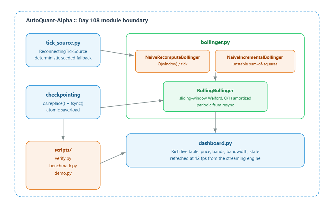
A live system does. The junior-engineer version of this lesson keeps a deque(maxlen=period) and, on every tick, slices it out and runs a full two-pass mean/variance computation from scratch: sum everything, compute the mean, sum every squared deviation from that mean, divide. Numerically this is fine — it’s the textbook stable formula. Architecturally it’s an O(window) operation running on every single tick. At period=20 and calm tick rates that’s invisible. The benchmark in this lesson’s workspace shows what happens as the window grows: naive recompute goes from roughly on par with a streaming update at period=20 to 32.7x slower at period=1000 on an 8,000-tick run. And window size isn’t the only multiplier — tick rate is the other one, and tick rate is not constant. It spikes exactly when a market is moving fast, which is exactly when your risk engine needs Bollinger Bands to keep up without falling behind the book.
The failure mode, and the trap inside the fix
The obvious fix is to make the per-tick cost O(1). Keep a running sum and a running sum-of-squares as the window slides — add the new tick, subtract the evicted one — and derive variance from the single-pass formula every stats course teaches: var = (sumsq - sum**2/n) / n. It’s four lines of arithmetic and it genuinely is O(1) per tick.
It is also numerically unsound, and the way it breaks is worse than slow: it’s silently wrong until it isn’t. Consider a $500,000 futures contract (large notional, not unusual) trading in a two-cent range. Every price in the window is around 50,000,000 cents. sum**2/n and sumsq are both on the order of 2.5 * 10^15, while the quantity that actually matters — the variance — lives around 10^0. float64 carries about 15-17 significant decimal digits. Subtracting two numbers that agree to 15 digits to recover a value 15 orders of magnitude smaller than either of them is the textbook definition of catastrophic cancellation: the subtraction can lose all its meaningful digits, and the result becomes float noise. On a long-running stream that noise doesn’t cancel out, it accumulates. The workspace’s test suite reproduces this directly (test_naive_incremental_diverges_or_fails _on_high_price_low_vol): feed the naive-incremental engine a tight-range, high-price sequence and it either reports a variance that’s visibly wrong or goes negative and blows up on sqrt(). Either failure mode is worse than the O(window) recompute it was supposed to replace, because the slow version at least gives you a correct number.
The AutoQuant-Alpha architecture