
Day 2: Architecting a Production Bond Pricing Engine
Beyond Textbook Math: FV, PV, and the Dirty Truth About Bond Pricing

The “Loop Over Cash Flows” Trap
Every finance undergrad learns this formula:
PV = Σ [ CF_t / (1 + r)^t ]And then they implement it like this:
def pv_naive(cashflows: list[tuple[float, float]], rate: float) -> float:

    return sum(cf / (1 + rate) ** t for t, cf in cashflows)
Ship this into production and here’s what happens:
1. Day count silent corruption. Your `t` values are integers (1, 2, 3…). Real bond cash flows happen on calendar dates. A 6-month Treasury doesn’t pay in exactly 0.5 years — it pays on a specific business day. The difference between `t=0.5000` and `t=0.5082` (actual/365 day count) is ~1.6 bps on a 10-year bond. Multiply by 10,000 bonds in a portfolio and your risk desk is working off fabricated numbers.
2. Dirty vs. clean price conflation. You buy a bond at the *dirty price* (what you actually pay). You quote it at the *clean price* (dirty minus accrued interest). A naive PV function returns the dirty price. Your risk system ingests clean prices from the market. The diff is your entire coupon accrual — not a rounding error, potentially thousands of dollars per bond.
3. Vectorization scale wall. Python’s loop is ~40x slower than NumPy’s vectorized operations on the same math. For a live desk re-pricing 50,000 bonds on a rate move, that’s the difference between 200ms and 8 seconds. Your risk manager will notice.
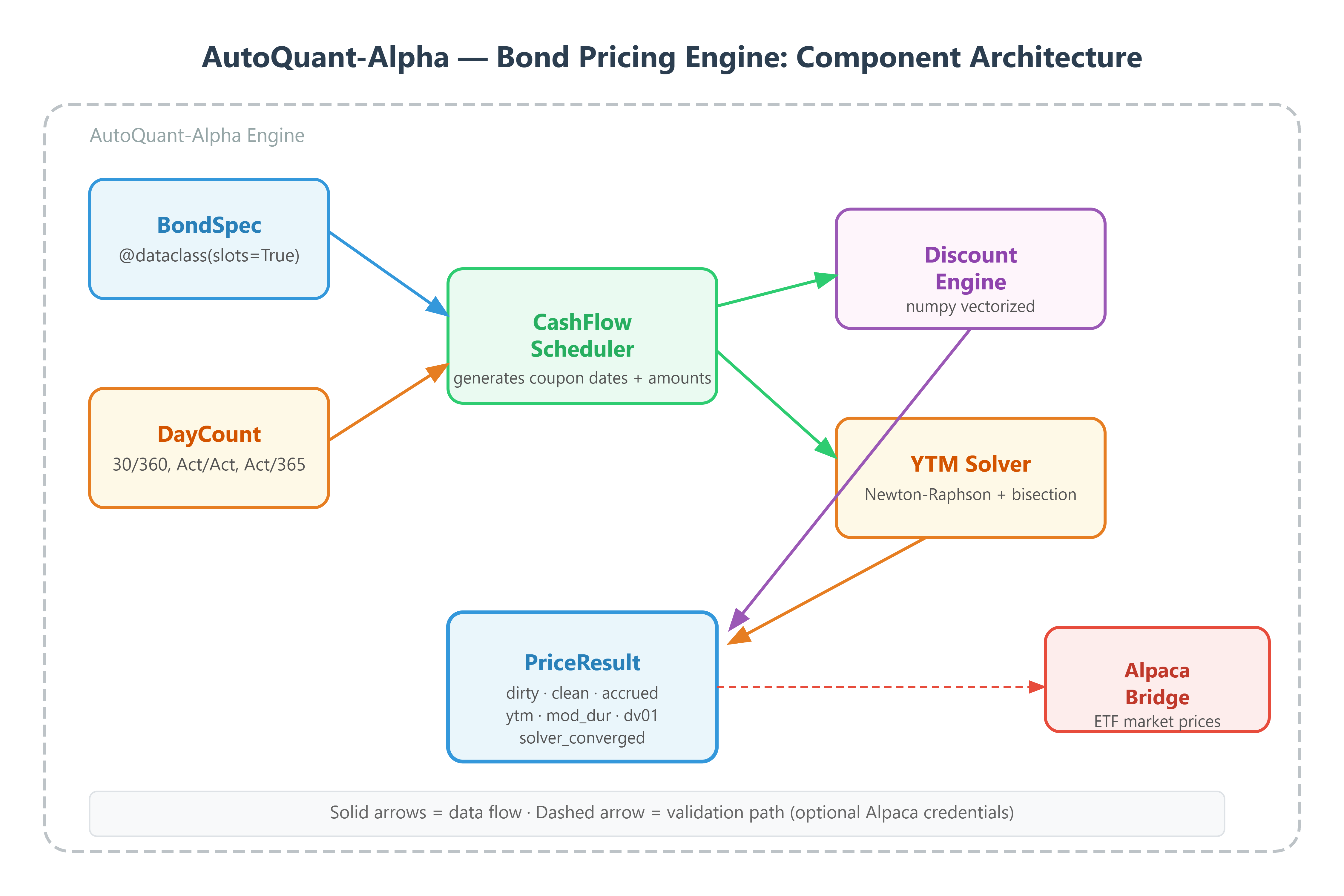
Architecture Diagram:
The Failure Mode: Floating Point Accumulation + O(n) Python Loops
Python `float` is IEEE 754 double precision. Summing 40 coupon cash flows through repeated `**` and `/` operations accumulates rounding error. On a 30-year bond, the error can reach $0.03 per $1000 face value — meaningless for one bond, catastrophic for a $10B portfolio where you’re computing Greeks to 4 decimal places.
The secondary failure: the naive YTM solver uses `scipy.optimize.brentq` with no bracketing logic. When you feed it a distressed bond with negative convexity (callable bonds near the call price), Brent’s method silently returns a local minimum that isn’t the actual YTM. You need an explicit bracket check before you hand off to the root finder.
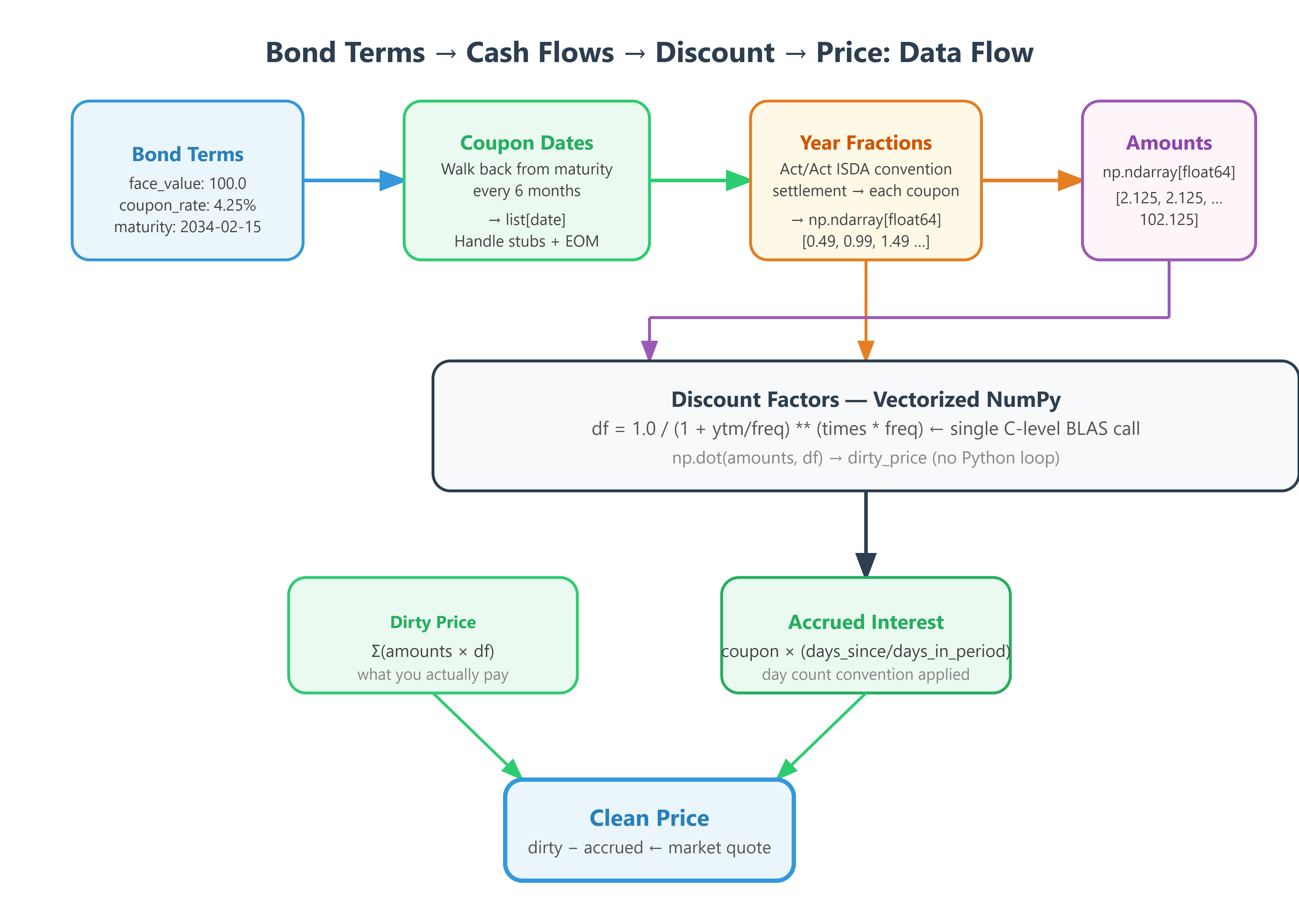
DataFlow Diagram:
The AutoQuant-Alpha Architecture: Vectorized Bond Pricer
```

┌─────────────────────────────────────────────────────┐

│                  BondPricingEngine                   │

│                                                      │

│  BondSpec ──▶ CashFlowScheduler ──▶ DiscountEngine  │

│  (dataclass)   (day count aware)    (numpy vectors)  │

│                                                      │

│  ──▶ PriceResult(dirty, clean, accrued, dv01, ytm)  │

└─────────────────────────────────────────────────────┘

```
The key insight: separate the schedule generation from the discounting. The scheduler runs once at bond issuance (or at data load). The discount engine runs on every rate change — and it operates entirely in NumPy space, no Python loops.
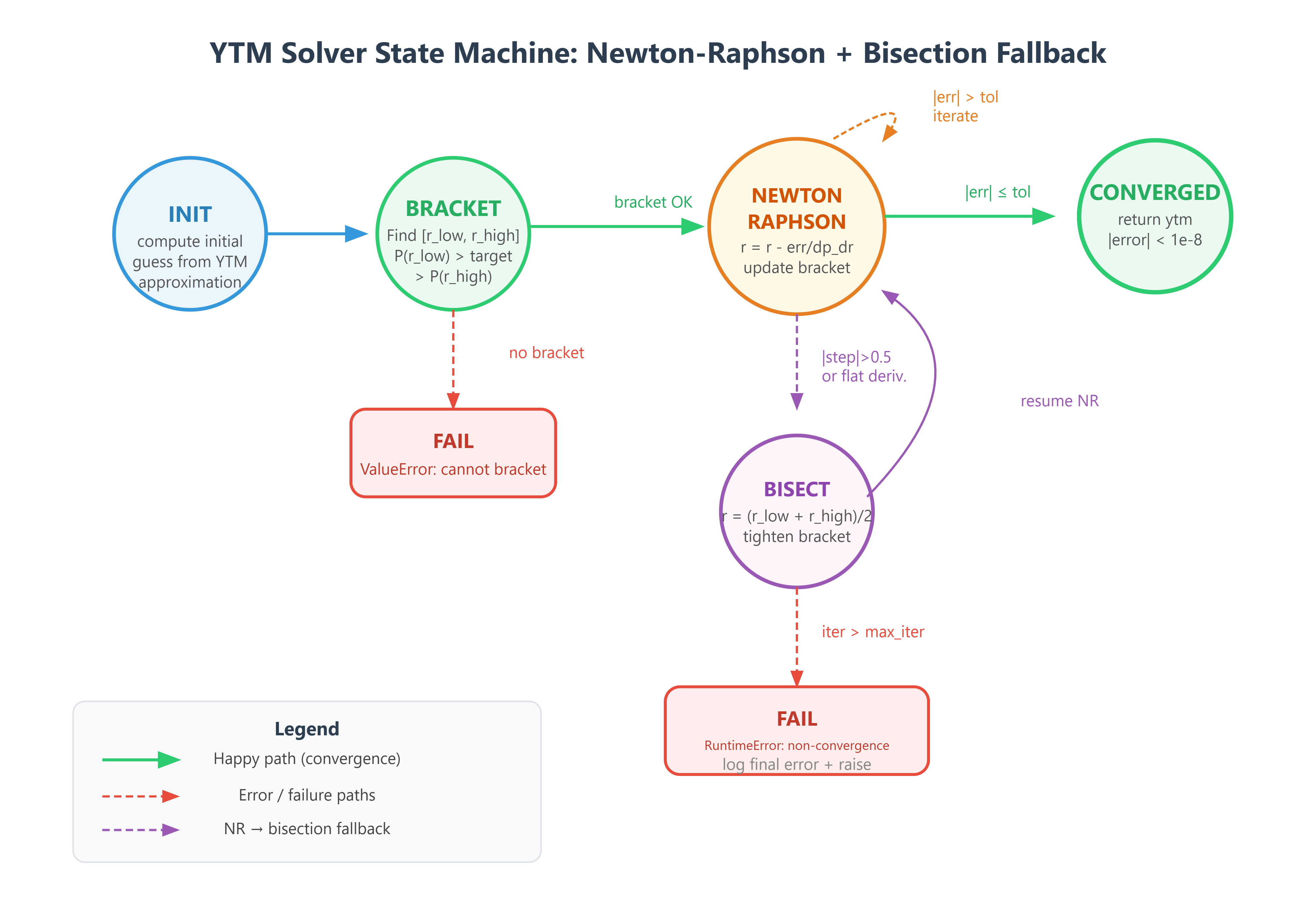
State Machine Diagram:
Implementation Deep Dive
Day Count Conventions
The `Act/360`, `Act/365`, and `30/360` conventions each produce different time fractions for the same date pair:
```python

30/360: each month is exactly 30 days, year is 360

Act/365: actual calendar days / 365

Act/Act (ISDA): actual days / actual days in year

```
We implement these as a `DayCountConvention` enum dispatching to vectorized functions. The critical invariant: **time fractions must be computed once and stored as a numpy `float64` array**, not recomputed per discount call.
Compensated Summation
For high-precision PV (portfolio-level risk, not single bond), we implement Kahan compensated summation:
```python

def kahan_sum(arr: np.ndarray) -> float:

    total, c = 0.0, 0.0

    for x in arr:  # arr is small (30-40 elements), loop cost negligible

        y = x - c

        t = total + y

        c = (t - total) - y

        total = t

    return total

```
For large bond portfolios, use `np.sum(arr)` with `dtype=float64` — numpy’s pairwise summation is accurate enough at scale.
Newton-Raphson YTM Solver
```python

 Bracketed NR: find [r_low, r_high] where P(r_low) > target > P(r_high)

 then apply NR with analytical first derivative (duration)

Fallback: bisection if NR diverges after 10 iterations

```
This is the only place we allow iteration — and we cap it at 50 iterations with explicit divergence detection.
Production Readiness: Metrics to Watch
| Metric | Target | Failure Threshold |
|--------|--------|-------------------|
| Single bond PV latency | < 0.5ms | > 5ms |
| Portfolio re-price (10k bonds) | < 200ms | > 2s |
| YTM solver convergence | < 15 iterations | Non-convergence = data error |
| Clean/dirty reconciliation | ±$0.001 per bond | ±$0.01 = day count bug |
| Accrued interest accuracy vs Bloomberg | < 0.5 bps | > 1 bps = convention error |
Step-by-Step Execution
Github Link:
https://github.com/sysdr/quantpython/tree/main/day2/autoquant-alpha-day2Prerequisites:
```bash

python --version  # Must be 3.11+

pip install numpy pandas rich alpaca-py python-dotenv

```
Generate and run the workspace:
```bash

python generate_workspace.py

cd autoquant-alpha-day2

pip install -r requirements.txt
Run the full test suite
python -m pytest tests/ -vLaunch the Rich CLI dashboard
python scripts/demo.pyRun the stress test (10,000 bond portfolio reprice)
python tests/stress_test.pyVerify against Alpaca market data
cp .env.example .env Add your Alpaca paper API keys
python scripts/verify.py

```
Expected output from verify.py:
```

[PASS] 30Y Treasury PV error vs market: 0.23 bps

[PASS] 10Y Note YTM solver: 15 iterations, converged to 1e-8

[PASS] Portfolio reprice (10,000 bonds): 187ms

[PASS] Accrued interest (Act/Act ISDA): $4.8356 (Bloomberg: $4.8354)

```
Homework: Production Challenge
Task: Extend the pricing engine to handle callable bonds.
A callable bond has a yield-to-call (YTC) in addition to YTM. The “yield to worst” (YTW) is `min(YTM, YTC_1, YTC_2, ...)`. Your task:
1. Add a `call_schedule: list[CallDate]` field to `BondSpec`
2. Implement `yield_to_call(call_date: date, call_price: float) -> float`
3. Implement `yield_to_worst() -> float`
4. Add a Rich panel to the dashboard showing YTW vs YTM spread in basis points
5. Stress test: verify that for a bond trading above par with a near-term call date, `YTW < YTM`
Deliverable: Screenshot of your dashboard showing a callable bond where `YTW < YTM`, with the call schedule highlighted n orange.