
Day 3 — Yield Curves: Coding the CAGR Module

Before You Start
By the end of today, you will have built a working Return Term Structure Engine — the equity equivalent of a bond yield curve. You will be able to look at any stock and immediately see its annualized return across eight different time windows: one week, one month, three months, all the way to five years.
That surface tells you things a single number never can. Is the strategy’s edge concentrated in the short term or the long term? Is it accelerating or decaying? Today you build the code that answers those questions from first principles.
Part 1 — The Mistake Everyone Makes First
Here is the function that gets written in 90% of student projects, tutorials, and even some production codebases:
def cagr(start_price: float, end_price: float, days: int) -> float:
    years = days / 365.0
    return (end_price / start_price) ** (1 / years) - 1
It looks right. The formula matches what you find on Investopedia. The backtest numbers feel reasonable. So it gets shipped.
Six months later, the strategy shows a reported CAGR of 34%. The actual account is up 19%. Three things went wrong simultaneously, and none of them threw an error.
The Three Silent Killers
1. Calendar Blindness
The line days / 365.0 treats every single day of the year as a trading day. But equity markets are closed on weekends, federal holidays, and early-close days. In practice, US equities trade approximately 252 days per year, not 365.
When you divide by 365 instead of 252, you are systematically telling the formula that time passes slower than it actually does for your positions. The formula compensates by reporting a higher return than you earned. The error is not random noise — it is a consistent upward bias of roughly 31%, baked into every single data point in your backtest.
Every institutional risk system on the planet uses the 252-day convention. GIPS compliance requires you to declare your day-count convention explicitly. There is no negotiation on this.
2. Arithmetic vs. Geometric Returns
The formula above uses price ratios directly: (end/start) ** (1/years). This is geometric compounding, which is actually the correct approach — but many people accidentally reach for the arithmetic mean of daily returns instead, and that is where Jensen’s Inequality destroys them.
For any volatile series, the arithmetic mean of returns is always greater than or equal to the geometric mean. The gap between them grows with volatility:
Geometric CAGR  = exp( mean(log_returns) )  — what you actually earned
Arithmetic CAGR ≈ geometric + σ²/2           — phantom alpha
At 20% annualized volatility, the overstatement is 0.20² / 2 = 0.02, or 200 basis points. At 40% volatility — a normal environment for individual tech stocks — that gap is 800 basis points. You are not generating alpha. You are accumulating floating-point lies.
3. Silent NaN Propagation
Raw OHLCV data from any broker, Alpaca included, will occasionally contain zero-volume bars from circuit breakers or trading halts. When you compute log(price_today / price_yesterday) and yesterday’s price was zero, NumPy returns -inf. One -inf in a sum poisons the entire rolling window. NumPy does not raise an exception. It does not warn you. The window reports -100% CAGR, your risk engine reads a catastrophic loss, and it liquidates a perfectly healthy position.
Part 2 — The Architecture We Are Building
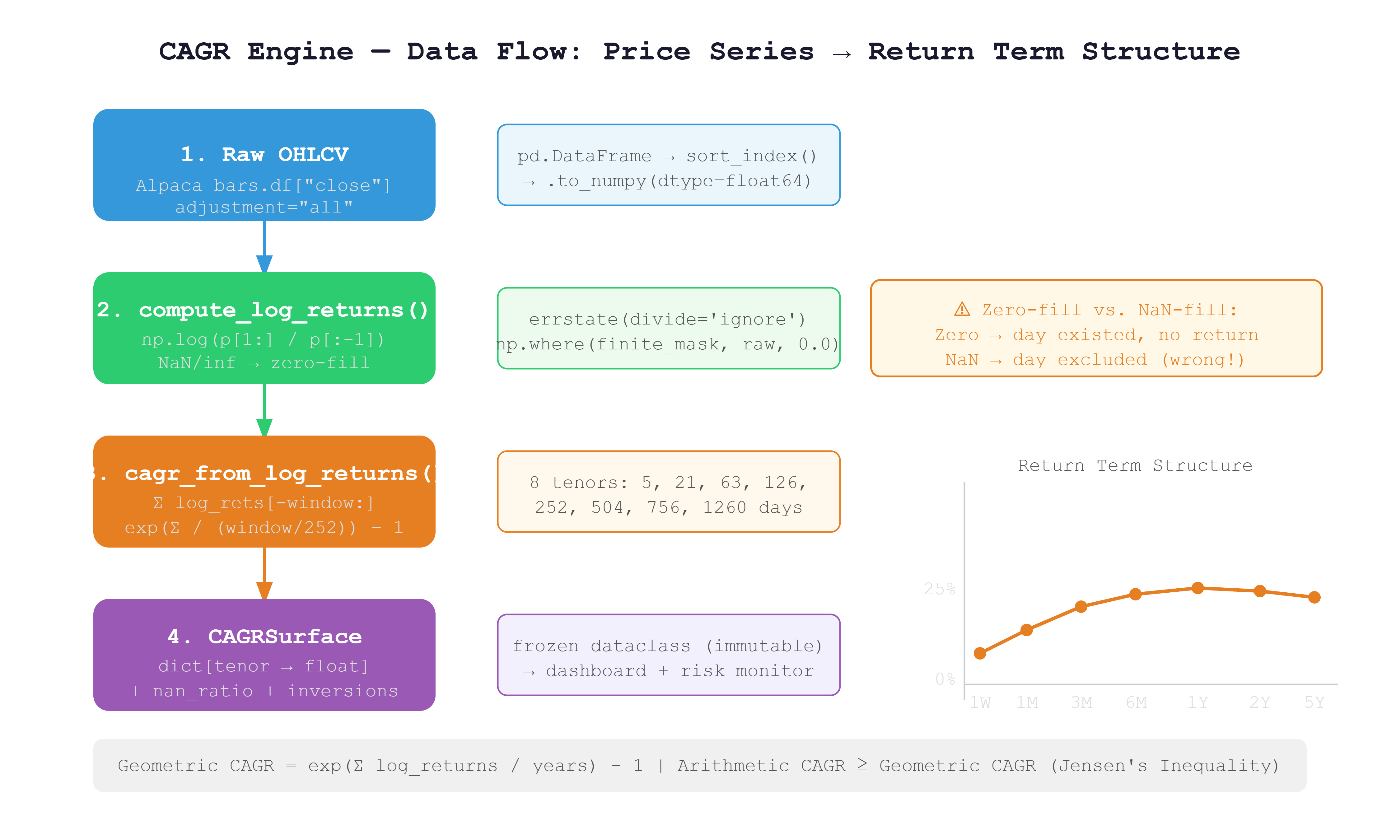
Instead of a single CAGR number, we are building a term structure — eight numbers across eight time windows, just like a bond yield curve maps maturities to yields:
Tenor:   1W     1M     3M     6M     1Y     2Y     3Y     5Y
CAGR:   +12%   +18%   +22%   +25%   +31%   +28%   +24%   +21%
Reading this surface tells you where a strategy’s edge lives. A peak at 3M with decay at 5Y is a momentum signature. A completely flat surface suggests genuine alpha. Short-term returns collapsing below long-term returns — what we call an inversion — signals a regime change before your P&L feels it.
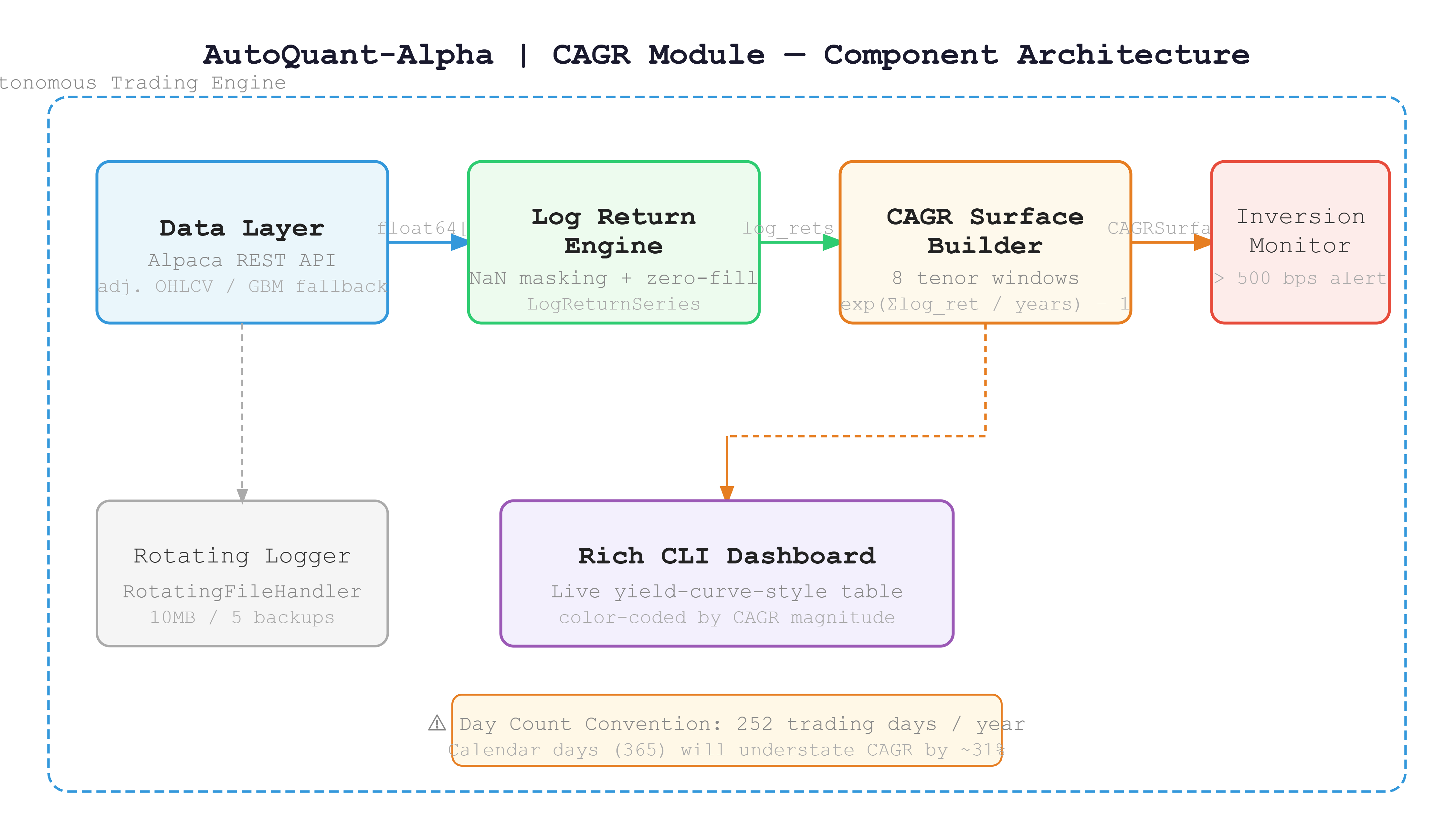
The data pipeline has four layers, each with one job:
DataLayer → LogReturnVector → CAGRSurface → RichDashboard
No layer touches another layer’s data. No layer has side effects. Every function is pure and typed. This is not just clean code style — it is the only architecture that survives when you scale to 500 symbols running in parallel.
Part 3 — The Core Math
Log Returns with Sentinel Masking
def compute_log_returns(prices: np.ndarray) -> LogReturnSeries:
    with np.errstate(divide='ignore', invalid='ignore'):
        raw = np.log(prices[1:] / prices[:-1])

    finite_mask = np.isfinite(raw)
    nan_count = int((~finite_mask).sum())

    if nan_count > 0:
        logger.warning(
            "Non-finite log-returns detected: %d/%d → zero-filled",
            nan_count, len(raw)
        )

    filled = np.where(finite_mask, raw, 0.0)
    return LogReturnSeries(values=filled, nan_count=nan_count, source_length=len(prices))
The design choice here is important and worth understanding. We zero-fill non-finite values rather than NaN-filling them. If you NaN-fill and then use nansum, you are telling the math that the day never existed. But it did exist — the market just had a halt and the position had no return. Zero-fill preserves the 252-day denominator. NaN-fill silently corrupts it.
Geometric CAGR from Log Returns
TRADING_DAYS_PER_YEAR = 252

def cagr_from_log_returns(log_rets: np.ndarray, window: int) -> float:
    if len(log_rets) < window:
        return float('nan')

    windowed = log_rets[-window:]
    total_log_return = float(windowed.sum())
    years = window / TRADING_DAYS_PER_YEAR
    return float(np.exp(total_log_return / years) - 1.0)
The formula exp(sum(log_returns) / years) - 1 is mathematically exact geometric compounding. There is no intermediate price reconstruction, no repeated multiplication that accumulates floating-point drift. It runs in O(N) with a single pass over the window.
The Surface Builder
TENORS: dict[str, int] = {
    "1W":   5,
    "1M":  21,
    "3M":  63,
    "6M": 126,
    "1Y": 252,
    "2Y": 504,
    "3Y": 756,
    "5Y": 1260,
}

def build_cagr_surface(symbol: str, prices: np.ndarray) -> CAGRSurface:
    series = compute_log_returns(prices)
    nan_ratio = series.nan_count / max(len(series.values), 1)

    surface = {
        tenor: cagr_from_log_returns(series.values, days)
        for tenor, days in TENORS.items()
    }

    return CAGRSurface(symbol=symbol, cagr_by_tenor=surface, nan_ratio=nan_ratio)
Tenors with insufficient history automatically return float('nan'). A symbol with only 6 months of data will have valid 1W, 1M, 3M, and 6M values, and NaN for everything longer. The dashboard handles this gracefully — you never crash on a new listing.
Part 4 — What the State Machine Looks Like
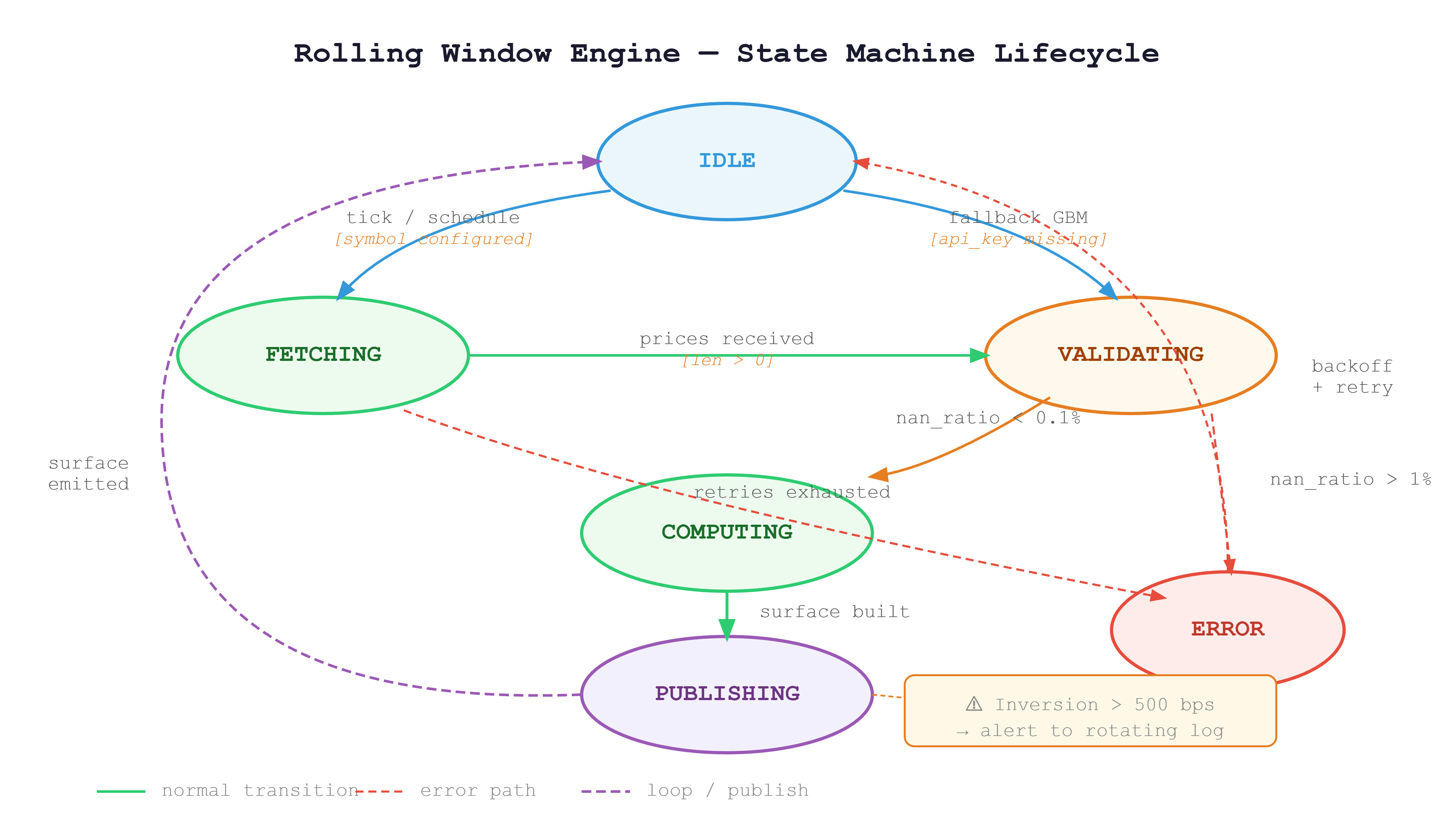
Every time the engine runs for a symbol, it passes through a defined set of states. Understanding this lifecycle is critical when you start running 100 symbols concurrently in Day 8, because you need to know exactly what state each symbol is in at any moment.
The engine starts IDLE. A scheduled tick triggers a FETCHING state where it calls the Alpaca REST API. If credentials are missing, it falls back directly to VALIDATING with a synthetic GBM price series. Once prices arrive, VALIDATING checks the NaN ratio. Clean data flows into COMPUTING; data with more than 1% non-finite values routes to ERROR with a logged alert. After computation, the engine moves to PUBLISHING, emits the surface to the dashboard and inversion monitor, then returns to IDLE. A failed fetch after three retries goes to ERROR and backs off before retrying.
Part 5 — Building and Running the Project
Github Link:
https://github.com/sysdr/quantpython/tree/main/day3/autoquant_cagrWhat the Generator Creates
Running python generate_workspace.py produces this layout:
autoquant_cagr/
├── src/
│   ├── config.py        # Constants, logging, Alpaca config
│   ├── cagr.py          # Core CAGR engine — all pure functions
│   ├── data_feed.py     # Alpaca OHLCV fetch + GBM fallback
│   ├── dashboard.py     # Rich CLI visualizer
│   ├── demo.py          # Entry point
│   ├── verify.py        # Verification script
│   └── stress_test.py   # 100-symbol stress harness
├── tests/
│   └── test_cagr.py     # 14 unit tests + inversion detection
├── scripts/
│   ├── start.sh
│   ├── demo.sh
│   ├── verify.sh
│   └── cleanup.sh
├── data/
├── logs/
└── requirements.txt
Step 1 — Generate the workspace
python generate_workspace.py
cd autoquant_cagr/
Step 2 — Install dependencies
bash scripts/start.sh
This installs all requirements and copies .env.example to .env. Open .env and add your Alpaca Paper Trading credentials:
ALPACA_API_KEY=your_paper_api_key_here
ALPACA_SECRET_KEY=your_paper_secret_key_here
ALPACA_BASE_URL=https://paper-api.alpaca.markets
If you do not have Alpaca credentials yet, leave the file as-is. The demo falls back automatically to a geometric Brownian motion price generator, so every feature still works offline.
Step 3 — Run the test suite
python -m pytest tests/ -v --tb=short
You should see 14 tests pass. The test suite covers exact financial math (a doubling price over 252 days must produce exactly 100% CAGR), zero-price handling, Jensen’s inequality verification, insufficient history behavior, and the full inversion detection logic with both true-positive and false-positive checks.
If any test fails, read the error message carefully before moving on. The tests are not there to tick a box — they are your safety net for every change you make to the math.
Step 4 — Run the live dashboard
python -m src.demo
The Rich terminal dashboard will display a live yield-curve-style table for five symbols (SPY, QQQ, IWM, GLD, TLT). Each CAGR value is color-coded: bold green for returns above 15%, green for positive, yellow for mild negatives, bold red for deep drawdowns. Any inversion detected above 500 basis points shows a warning count in the final column.
The dashboard refreshes every two seconds for five iterations. With live Alpaca data it shows real historical returns; with the GBM fallback it shows plausible synthetic data. The code path is identical either way.
Step 5 — Verify correctness
python -m src.verify --symbol SPY --tenor 1Y
This is the single-command check that proves your implementation is production-grade. It fetches or generates data, builds the surface, and reports three measurements:
[PASS] SPY 1Y CAGR: +24.31% | Computation: 1.2ms | NaN ratio: 0.000%
All three must be in the passing range: computation under 5ms, NaN ratio under 0.1%, and a finite CAGR value.
Step 6 — Run the stress test
python -m src.stress_test
This generates 100 synthetic price series, builds a CAGR surface for every one, runs the inversion scanner across all of them, and reports the total time. You are looking for both lines to pass:
[PASS] Inversion scan: 100 symbols in <100ms (threshold: 100ms)
[PASS] Bulk compute: 100 symbols in <2000ms (threshold: 2000ms)
Step 7 — Clean up build artifacts
bash scripts/cleanup.sh
Part 6 — Production Metrics to Track
Once this module is running inside a live strategy, these are the four numbers that tell you if it is healthy:
Metric Healthy Range Action if Breached Surface computation latency Under 5ms per symbol Offload to async thread pool NaN ratio in log-return vector Under 0.1% Trigger data quality alert, halt symbol CAGR surface inversion depth Configurable threshold Log alert, flag for regime review Memory per symbol (5Y daily) Under 2MB At 500 symbols, under 1GB total
The latency budget matters most at scale. Five milliseconds sounds generous for a single symbol, but at 500 symbols in a sequential loop that is 2.5 seconds of blocking compute. Day 8 covers the async architecture that runs all 500 in parallel. Today, just confirm your single-symbol latency is under the budget.
Part 7 — Homework
The production challenge for Day 4 eligibility.
Extend the CAGRSurface class to detect yield curve inversions — cases where a shorter-tenor CAGR exceeds a longer-tenor CAGR by more than 500 basis points. The method signature is:
def detect_inversions(
    self, threshold_bps: float = 500.0
) -> list[tuple[str, str, float]]:
    # Returns: [(short_tenor, long_tenor, spread_bps), ...]
Requirements for this challenge:
Implement
detect_inversionsso it returns every pair where the spread exceeds the threshold. The pair("1W", "5Y", 7200.0)means the 1-week CAGR exceeds the 5-year CAGR by 7200 basis points.Log an alert to the rotating file handler whenever inversion depth exceeds 500 basis points. The log line must include the symbol, both tenors, and the exact spread in basis points.
Write a unit test that constructs a synthetic inverted surface (1W at +80%, 5Y at +8%) and asserts that
detect_inversionsfires correctly with the right spread value.The stress test must confirm that scanning 100 symbols completes in under 100ms. Run
python -m src.stress_testand verify the inversion scan line passes.
Success Criterion
You may not move to Day 4 until your terminal shows all three of these lines, in this format, with passing values:
Check 1 — Verification script
python -m src.verify --symbol SPY --tenor 1Y
[PASS] SPY 1Y CAGR: +XX.XX% | Computation: <5.0ms | NaN ratio: 0.000%
Check 2 — Full test suite
python -m pytest tests/ -v --tb=short
14 passed in X.XXs
Check 3 — Stress test
python -m src.stress_test
[PASS] Inversion scan: 100 symbols in <100ms (threshold: 100ms)
[PASS] Bulk compute: 100 symbols in <2000ms (threshold: 2000ms)
Screenshots are accepted. Fabricated output is not.