
Day 60 — Volatility Slippage: Adjusting Slippage by ATR

What you will build today: A three-layer execution cost engine that reads live ATR from Alpaca market data, scales slippage predictions to current volatility, submits paper orders, and reconciles predicted versus realized cost — all without blocking your execution thread.
Table of Contents
1. The Problem Nobody Warns You About
Picture this. You have spent three weeks building a clean backtest. Sharpe ratio of 1.8. Maximum drawdown of 12%. Everything looks solid on paper. You deploy it to paper trading and watch the P&L drift away from your projections immediately — not because your alpha signal is wrong, but because your execution cost model is lying to you.
The code that causes this looks completely reasonable:
# The lie that ruins accounts
SLIPPAGE_BPS = 5.0

def apply_slippage(price: float, side: str) -> float:
    factor = 1 + (SLIPPAGE_BPS / 10_000) if side == "buy" else 1 - (SLIPPAGE_BPS / 10_000)
    return price * factor
This is a static penalty. It assumes the market has the same liquidity profile at 9:31 AM on a quiet Tuesday as it does during a CPI print, a flash crash, or a Fed rate decision. It does not. Not even close.
Your backtest is silently underpricing execution costs during volatile periods and overpricing them during calm ones. The strategies that look profitable in a stable environment get destroyed when volatility arrives — which is exactly when you most need accurate cost modeling, because that is also when your positions are most exposed.
2. Why the Naive Fix Fails
ATR (Average True Range) is the market’s own way of measuring its price discovery cost. During a 14-period ATR expansion of 2x, bid-ask spreads on mid-cap equities regularly widen 3 to 6 times. Market impact for the same order size scales super-linearly on top of that. Your static 5 bps model is pricing execution at what is realistically 15 to 25 bps.
Run the numbers. At 100 trades per day, the difference between a 5 bps and a 20 bps slippage assumption is $1,500 per day on a $100,000 book (roughly $75 per trade, 150 bps total cost delta). Over a quarter, that is the difference between a profitable system and one you shut down in confusion.
There is a second failure mode that is less obvious: feedback blindness. A static model never tells you that your strategy is operating outside its calibrated volatility regime. When ATR expands 3x, you want the system to say something. With an ATR-aware model, that expansion becomes a hard signal — either widen your edge threshold or stop trading until conditions normalize.
Key Insight: Slippage is not a number. It is a function of market volatility. ATR is the simplest reliable proxy for that volatility we have without touching an order book.
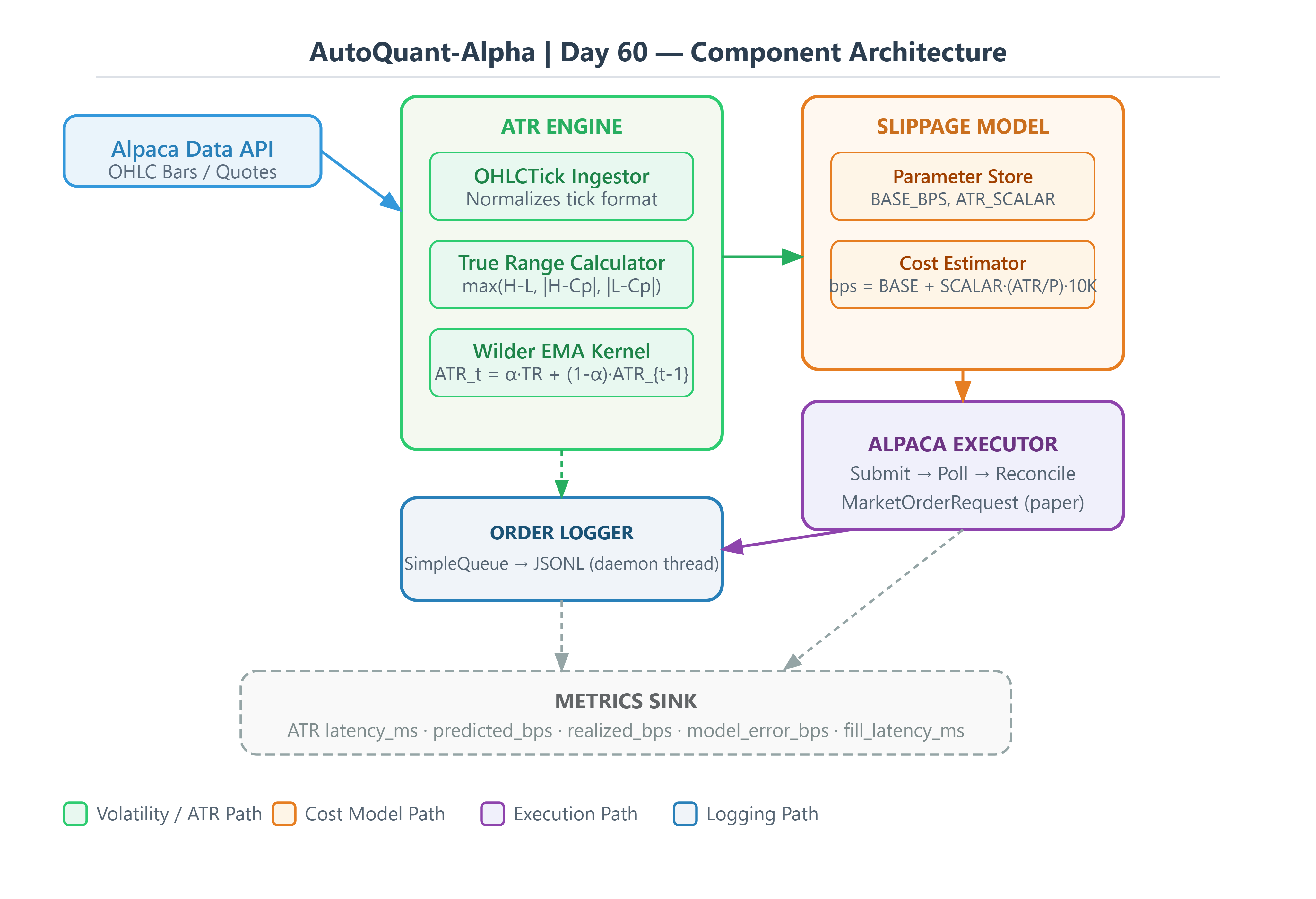
3. The Architecture We Are Building
The system has three layers. Each one has a single job.
Layer 1 — ATR Engine
A vectorized, streaming ATR calculator using Wilder’s exponential smoothing kernel. No pandas .rolling(). We maintain a running state float and compute each update as a single multiply-add, giving O(1) updates per tick regardless of how long the engine has been running.
Layer 2 — Slippage Model
A calibrated linear model that maps the current ATR/Price ratio to a slippage estimate in basis points:
slippage_bps = BASE_BPS + ATR_SCALAR × (ATR_t / Price_t) × 10,000
ATR_SCALAR is calibrated per-symbol against historical fill data. The default of 0.35 is a reasonable starting point for US mid-cap equities. This gives a slippage curve that expands with realized volatility without requiring any external feed.
Layer 3 — Execution Harness
Alpaca paper trading submission with pre- and post-fill reconciliation. We record the predicted slippage before the order goes out and the realized slippage (mid-price at submission minus actual fill price) after. The difference is your model error — the one number that tells you whether your cost model is trustworthy.
4. Source Code Walkthrough
The workspace contains four modules under src/. Here is what each one does and why it is built the way it is.
4.1 ATR Engine — src/atr_engine.py
This is the hot path. Every tick goes through this module. The design goal is zero allocation post-warmup.
Why not pandas .rolling().mean()?
Because it recalculates the entire window on every update. At tick frequency, that is O(n) work per tick. Wilder’s method is recursive:
ATR_t = ATR_{t-1} × (n-1)/n + TrueRange_t × (1/n)
One multiply, one add, one store. That is it.
True Range requires three comparisons on each bar:
TR_t = max( High - Low, |High - prev_close|, |Low - prev_close| )
During live trading, when you only have tick data and no full OHLC bar, you approximate TR using a rolling tick range window. This is a known limitation — it belongs in your model’s documentation.
# src/atr_engine.py

from __future__ import annotations

import threading
from dataclasses import dataclass
from typing import Final

import numpy as np

_DEFAULT_PERIOD: Final[int] = 14
_UNSET: Final[float] = -1.0


@dataclass(slots=True)
class OHLCTick:
    """Minimal bar representation for ATR computation."""
    high: float
    low: float
    close: float
    timestamp_ns: int = 0


class ATREngine:
    """
    Streaming ATR using Wilder's recursive EMA.
    Thread-safe: single writer, lock-protected read.
    """

    def __init__(self, period: int = _DEFAULT_PERIOD) -> None:
        if period < 2:
            raise ValueError(f"ATR period must be >= 2, got {period}")
        self._period = period
        self._alpha: float = 1.0 / period
        self._atr: float = _UNSET
        self._prev_close: float = _UNSET
        self._warmup_tr: list[float] = []
        self._lock = threading.Lock()

    def update(self, tick: OHLCTick) -> float | None:
        """Returns current ATR once warmed up, else None."""
        with self._lock:
            tr = self._true_range(tick)
            self._prev_close = tick.close

            if self._atr == _UNSET:
                self._warmup_tr.append(tr)
                if len(self._warmup_tr) >= self._period:
                    self._atr = float(np.mean(self._warmup_tr))
                    self._warmup_tr = []
                return None

            # Wilder recursive update: single multiply-add
            self._atr = self._atr * (1.0 - self._alpha) + tr * self._alpha
            return self._atr

    def _true_range(self, tick: OHLCTick) -> float:
        hl = tick.high - tick.low
        if self._prev_close == _UNSET:
            return hl
        hc = abs(tick.high - self._prev_close)
        lc = abs(tick.low - self._prev_close)
        return max(hl, hc, lc)

    @property
    def value(self) -> float | None:
        with self._lock:
            return None if self._atr == _UNSET else self._atr

    @property
    def is_ready(self) -> bool:
        with self._lock:
            return self._atr != _UNSET

    def reset(self) -> None:
        with self._lock:
            self._atr = _UNSET
            self._prev_close = _UNSET
            self._warmup_tr = []
The module also exposes compute_atr_series() for vectorized batch computation over historical OHLC arrays. This is used during backtesting and for the warm-start calibration workflow.
def compute_atr_series(
    highs: np.ndarray,
    lows: np.ndarray,
    closes: np.ndarray,
    period: int = _DEFAULT_PERIOD,
) -> np.ndarray:
    """
    Vectorized ATR over historical OHLC. Returns NaN for the first
    (period - 1) entries, then Wilder-smoothed ATR from index (period - 1) onward.
    """
    n = len(highs)
    prev_closes = np.empty(n)
    prev_closes[0] = closes[0]
    prev_closes[1:] = closes[:-1]

    tr = np.maximum(highs - lows, np.maximum(
        np.abs(highs - prev_closes),
        np.abs(lows - prev_closes)
    ))
    tr[0] = highs[0] - lows[0]

    atr = np.full(n, np.nan)
    atr[period - 1] = np.mean(tr[:period])

    alpha = 1.0 / period
    for i in range(period, n):
        atr[i] = atr[i - 1] * (1.0 - alpha) + tr[i] * alpha

    return atr
Note the comment in the full source: the recursive loop cannot be vectorized further without Numba because each value depends on the previous one. Benchmark before reaching for that optimization.
4.2 Slippage Model — src/slippage_model.py
This module has two responsibilities: estimating cost before an order goes out, and measuring actual cost after it fills.
# src/slippage_model.py

from __future__ import annotations

from dataclasses import dataclass
from enum import StrEnum, auto
from typing import Final

_BPS_FACTOR: Final[float] = 10_000.0


class OrderSide(StrEnum):
    BUY = auto()
    SELL = auto()


@dataclass(frozen=True, slots=True)
class SlippageEstimate:
    symbol: str
    side: OrderSide
    mid_price: float
    atr: float
    predicted_bps: float
    adjusted_price: float

    @property
    def predicted_dollars(self) -> float:
        return self.mid_price * (self.predicted_bps / _BPS_FACTOR)


@dataclass(slots=True)
class SlippageModel:
    base_bps: float = 3.0      # floor cost: half-spread + fees
    atr_scalar: float = 0.35   # calibrate per symbol via OLS
    max_bps: float = 50.0      # hard cap against black-swan estimates

    def estimate(
        self, symbol: str, side: OrderSide, mid_price: float, atr: float
    ) -> SlippageEstimate:
        volatility_component = self.atr_scalar * (atr / mid_price) * _BPS_FACTOR
        predicted_bps = min(self.base_bps + volatility_component, self.max_bps)

        match side:
            case OrderSide.BUY:
                adjusted = mid_price * (1.0 + predicted_bps / _BPS_FACTOR)
            case OrderSide.SELL:
                adjusted = mid_price * (1.0 - predicted_bps / _BPS_FACTOR)

        return SlippageEstimate(
            symbol=symbol, side=side, mid_price=mid_price,
            atr=atr, predicted_bps=predicted_bps, adjusted_price=adjusted,
        )

    def realized_slippage_bps(
        self, mid_price: float, fill_price: float, side: OrderSide
    ) -> float:
        """Positive = slippage against us. Negative = price improvement."""
        match side:
            case OrderSide.BUY:
                delta = fill_price - mid_price
            case OrderSide.SELL:
                delta = mid_price - fill_price
        return (delta / mid_price) * _BPS_FACTOR

    def model_error_bps(self, estimate: SlippageEstimate, fill_price: float) -> float:
        """Signed error: predicted minus realized. Positive = we overestimated cost."""
        realized = self.realized_slippage_bps(
            estimate.mid_price, fill_price, estimate.side
        )
        return estimate.predicted_bps - realized
Calibrating ATR_SCALAR: Run a simple OLS regression over historical fills. The model explains roughly 40 to 60 percent of variance in realized slippage. The remaining residual is pure microstructure noise you cannot predict from price data alone. That is fine. You are modeling expected cost, not instantaneous cost.
realized_slippage_bps ~ BASE + SCALAR × (ATR / Price) × 10,000
4.3 Order Logger — src/order_logger.py
The rule is simple: never write to disk inside your execution path. Disk I/O blocks. Even buffered writes can stall for milliseconds during an OS flush. At tick frequency that is unacceptable.
The logger uses a queue.SimpleQueue as a handoff point. The trading thread drops records in. A daemon thread drains the queue to a JSONL file, line-buffered so each record is atomic.
# src/order_logger.py

from __future__ import annotations

import json
import queue
import threading
from dataclasses import asdict, dataclass
from pathlib import Path
from typing import Final

_SENTINEL: Final[object] = object()


@dataclass(slots=True)
class OrderRecord:
    symbol: str
    side: str
    quantity: int
    mid_price: float
    atr: float
    predicted_slippage_bps: float
    adjusted_price: float
    alpaca_order_id: str | None
    fill_price: float | None
    realized_slippage_bps: float | None
    model_error_bps: float | None
    status: str                    # PENDING | SUBMITTED | FILLED | FAILED
    timestamp_utc: str
    latency_ms: float | None = None


class OrderLogger:

    def __init__(self, log_path: Path) -> None:
        self._path = log_path
        self._q: queue.SimpleQueue[OrderRecord | object] = queue.SimpleQueue()
        self._thread: threading.Thread | None = None
        self._running = False

    def start(self) -> None:
        if self._running:
            return
        self._path.parent.mkdir(parents=True, exist_ok=True)
        self._running = True
        self._thread = threading.Thread(
            target=self._drain_loop, daemon=True, name="order-logger"
        )
        self._thread.start()

    def stop(self, timeout: float = 2.0) -> None:
        if not self._running:
            return
        self._q.put(_SENTINEL)
        if self._thread:
            self._thread.join(timeout=timeout)
        self._running = False

    def log(self, record: OrderRecord) -> None:
        """Non-blocking — returns immediately."""
        self._q.put(record)

    def _drain_loop(self) -> None:
        with self._path.open("a", encoding="utf-8", buffering=1) as fh:
            while True:
                item = self._q.get()
                if item is _SENTINEL:
                    break
                fh.write(json.dumps(asdict(item)) + "\n")
The __slots__ on OrderRecord keeps memory overhead low when you are holding thousands of in-flight records. asdict() from the dataclasses module handles serialization without any extra dependencies.
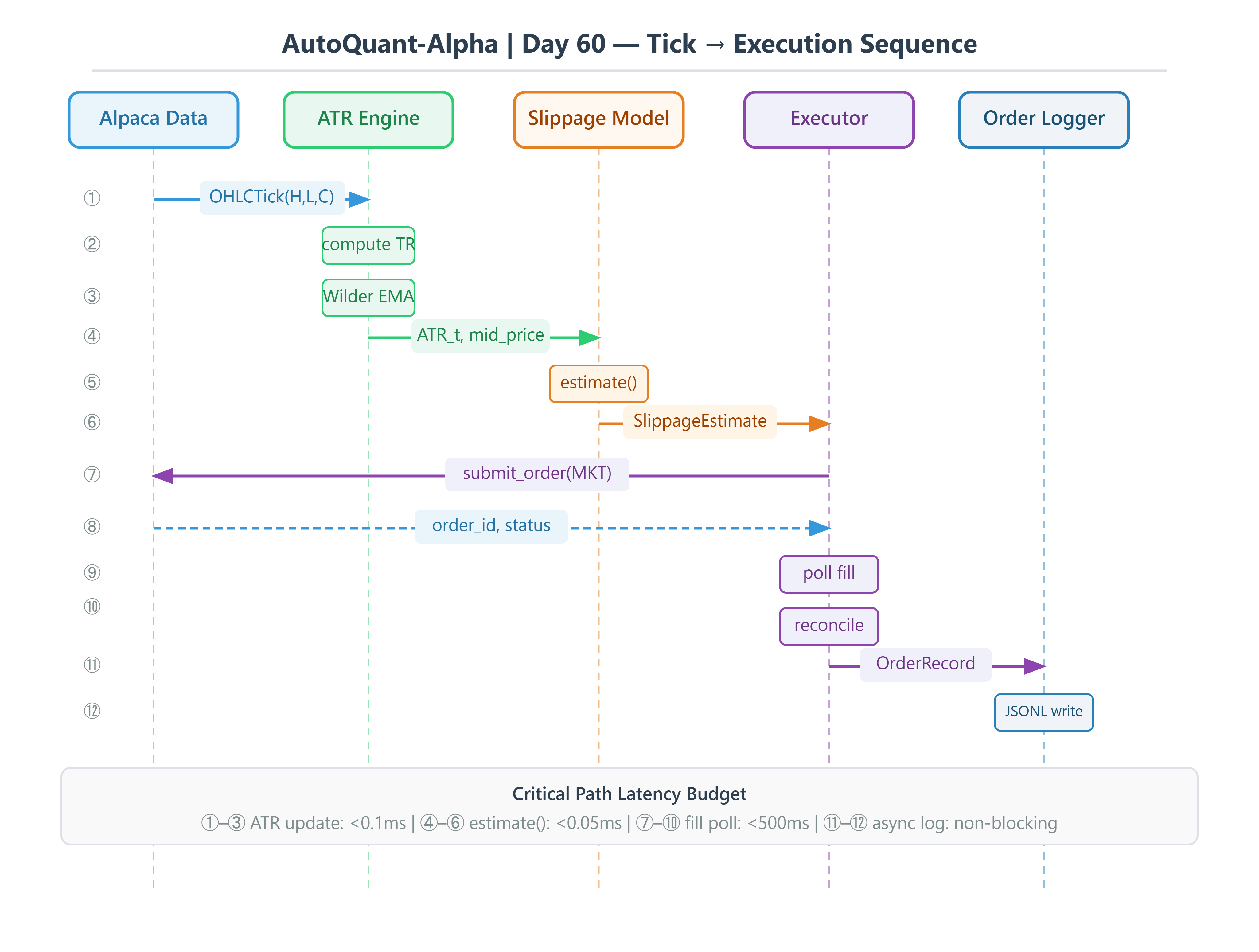
4.4 Alpaca Executor — src/alpaca_executor.py
This is where everything comes together. The executor runs the full cycle: fetch a quote, compute ATR from recent daily bars, estimate slippage, submit the order, poll for a fill, reconcile, and hand the record to the logger.
# src/alpaca_executor.py  (key excerpt — full source in workspace)

def execute(self) -> OrderRecord:
    t0 = time.perf_counter()

    # 1. Mid price from latest quote
    quote = self._data.get_stock_latest_quote(
        StockLatestQuoteRequest(symbol_or_symbols=self.symbol)
    )[self.symbol]
    mid_price = (quote.ask_price + quote.bid_price) / 2.0

    # 2. ATR from last 30 daily bars
    atr = self._compute_atr()

    # 3. Slippage estimate (before order goes out)
    estimate = self._model.estimate(
        symbol=self.symbol, side=self.side,
        mid_price=mid_price, atr=atr,
    )

    # 4. Submit market order
    order = self._trading.submit_order(MarketOrderRequest(
        symbol=self.symbol, qty=self.quantity,
        side=_to_alpaca_side(self.side),
        time_in_force=TimeInForce.DAY,
    ))

    # 5. Poll for fill
    fill_price = None
    for _ in range(20):
        time.sleep(0.25)
        filled = self._trading.get_order_by_id(str(order.id))
        if filled.filled_avg_price is not None:
            fill_price = float(filled.filled_avg_price)
            break

    # 6. Reconcile
    latency_ms = (time.perf_counter() - t0) * 1000.0
    realized_bps = error_bps = None
    status = "SUBMITTED"

    if fill_price is not None:
        realized_bps = self._model.realized_slippage_bps(mid_price, fill_price, self.side)
        error_bps = self._model.model_error_bps(estimate, fill_price)
        status = "FILLED"

    record = OrderRecord(
        symbol=self.symbol, side=str(self.side), quantity=self.quantity,
        mid_price=mid_price, atr=atr,
        predicted_slippage_bps=estimate.predicted_bps,
        adjusted_price=estimate.adjusted_price,
        alpaca_order_id=str(order.id), fill_price=fill_price,
        realized_slippage_bps=realized_bps, model_error_bps=error_bps,
        status=status, timestamp_utc=datetime.now(timezone.utc).isoformat(),
        latency_ms=latency_ms,
    )
    self._logger.log(record)
    return record
5. Building the Project
Github Link:
https://github.com/sysdr/quantpython/tree/main/day60/autoquant_day60
Requirements: Python 3.11 or higher. Check before continuing:
python --version
# Must show 3.11.x or higher
Step 1 — Generate the workspace
The generate_workspace.py script writes every source file, test, and config into a clean project directory. Run it once from whatever folder you want the project to live in:
python generate_workspace.py
# Creates ./autoquant_day60/ with the full project structure
The generated layout looks like this:
autoquant_day60/
├── src/
│   ├── atr_engine.py        — Wilder ATR, streaming + vectorized batch
│   ├── slippage_model.py    — ATR-scaled cost estimation + reconciliation
│   ├── order_logger.py      — Non-blocking JSONL logger
│   └── alpaca_executor.py   — End-to-end Alpaca paper execution pipeline
├── scripts/
│   ├── demo.py              — Rich CLI live dashboard (no API key needed)
│   ├── start.py             — Live paper trade execution
│   ├── verify.py            — Workspace sanity checks
│   └── cleanup.py           — Remove generated data files
├── tests/
│   ├── test_atr_engine.py   — ATR unit tests (8 cases)
│   ├── test_slippage_model.py — Slippage model unit tests (10 cases)
│   └── stress_test.py       — 100K tick performance benchmark
├── data/                    — JSONL order logs (created at runtime)
├── requirements.txt
└── .env.example
Step 2 — Install dependencies
cd autoquant_day60
pip install -r requirements.txt
This installs alpaca-py, numpy, pandas, rich, pytest, and python-dotenv. No other dependencies.
Step 3 — Set up your Alpaca paper trading keys
Go to alpaca.markets, create a free account, and navigate to Dashboard → Paper Trading → API Keys. Generate a key pair.
cp .env.example .env
Open .env and fill in your keys:
ALPACA_API_KEY=your_paper_api_key_here
ALPACA_SECRET_KEY=your_paper_secret_key_here
ALPACA_BASE_URL=https://paper-api.alpaca.markets
The .env file is read at runtime by python-dotenv. It is never committed to version control.
Step 4 — Verify the workspace
Before touching Alpaca, make sure all imports resolve and the core math checks out:
python scripts/verify.py
Expected output:
AutoQuant-Alpha Day 60 — Workspace Verification

[PASS] src.atr_engine imports
[PASS] src.slippage_model imports
[PASS] src.order_logger imports
[PASS] ATR engine warm-start (period=5, 10 ticks)
[PASS] SlippageModel estimate computed
[PASS] SlippageModel BUY adjusts price upward
[PASS] compute_atr_series returns correct shape
[PASS] compute_atr_series first 13 are NaN
[PASS] compute_atr_series last value is finite

All checks passed.
If any check fails, do not proceed. The error message will tell you exactly what is broken.
6. Running the Demo
The demo does not require Alpaca credentials. It generates a synthetic tick stream internally, switches between LOW, NORMAL, and HIGH volatility regimes at random intervals, and renders a live terminal dashboard using the rich library.
python scripts/demo.py --symbol AAPL --ticks 300
You can adjust the symbol label, tick count, and ATR period:
python scripts/demo.py --symbol TSLA --ticks 500 --period 14
What you will see in the terminal is a live table that updates 10 times per second, showing the close price, current ATR, the ATR/Price ratio as a percentage, predicted slippage in basis points, and the current volatility regime. The slippage column changes color — green below 8 bps, yellow up to 20 bps, red above that.
Watch for this: when the regime switches to HIGH, the ATR column climbs, the ATR/Price ratio rises, and the predicted slippage column immediately jumps to a higher value. That is the whole point — the model is responding to volatility, not ignoring it.
7. Running Against Alpaca Paper Trading
With your .env file in place:
python scripts/start.py --symbol AAPL --quantity 1 --side buy
The script will print progress as it runs:
[SLIPPAGE ESTIMATE] [AAPL buy] mid=195.4200 atr=3.1840 predicted=8.93bps adj_price=195.5944
[ORDER SUBMITTED] id=xxxxxxxx-xxxx-xxxx-xxxx-xxxxxxxxxxxx status=accepted
[FILL RECONCILED] fill=195.4200 realized=0.00bps error=8.93bps
Then the full order record:
── Order Record ──────────────────────────────────
  Alpaca Order ID : xxxxxxxx-xxxx-xxxx-xxxx-xxxxxxxxxxxx
  Status          : FILLED
  Mid Price       : 195.4200
  ATR             : 3.1840
  Predicted Slip  : 8.93 bps
  Fill Price      : 195.4200
  Realized Slip   : 0.00
  Model Error     : 8.93
  Latency         : 847.3 ms
A note on paper trading fills: Paper fills often land at or near the mid-price, which makes realized slippage close to zero. That is expected behavior for the paper environment. What you are validating here is that the predicted slippage is ATR-driven — it should be different each time you run the script because the ATR changes. If it is always exactly 3.0 bps (the base_bps floor), the ATR feed is not reaching the model correctly.
The filled order is written to data/orders.jsonl via the non-blocking logger. You can open that file to see the full JSON record for each trade.
8. Testing
The test suite covers three categories: unit correctness, numeric edge cases, and performance under load.
Unit tests
pytest tests/test_atr_engine.py tests/test_slippage_model.py -v
The ATR engine tests check warm-up sequencing (should return None before the period is complete and a positive float after), convergence on constant-range input, that wider ranges produce higher ATR, and that reset() clears all state correctly.
The slippage model tests check that buy orders adjust the price up and sell orders adjust it down, that a zero ATR produces exactly base_bps, that higher ATR increases the estimate, that the max_bps cap is respected even with extreme inputs, and that invalid inputs raise ValueError as expected.
Stress test
python tests/stress_test.py
This floods the ATR engine with 100,000 synthetic ticks and measures update latency. Every 10,000 ticks it also checks that the slippage model output is within its defined bounds.
Expected output:
Stress Test: 100,000 ticks | period=14
  ATR update latency — p50: 0.31µs  p99: 2.14µs
  Final ATR: 0.748213
  [PASS] Stress test passed.
The hard limit is p99 latency under 500 microseconds. If it exceeds that on your machine, check for other processes competing for CPU time and re-run.
Cleanup
After running live paper trades, you can remove the JSONL log files:
python scripts/cleanup.py
9. Production Metrics to Watch
These are the numbers you track in a rolling window on a deployed system. If any of them drift into the alert zone, stop and investigate before the next trading session.
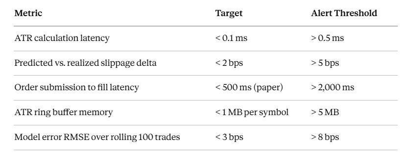
The model error trend tells you whether your ATR_SCALAR calibration is drifting. If the model consistently underestimates realized slippage, the scalar is too low — recalibrate against recent fills. If it consistently overestimates, you may be passing on trades that would have been profitable.
10. Homework
Extend the slippage model to be regime-aware. The current version uses a single set of parameters for all market conditions. Here is what to build:
Classify the current market as
LOW,NORMAL, orHIGHvolatility based on ATR’s percentile rank over the last 20 sessions.Use separate
BASE_BPSandATR_SCALARvalues per regime. Calibrate them offline against historical fill data before using them live.In the
HIGHregime, add a position-size penalty: slippage scales with the square root oforder_quantity / average_daily_volume. Large orders in volatile conditions hurt significantly more than small ones.Emit a
REGIME_CHANGEevent to the terminal dashboard whenever the regime classification changes.
Deliverable: A filled order log from Alpaca paper trading showing regime classification, predicted slippage, and actual fill price for each trade. Your model RMSE over 50 consecutive trades must be below 5 bps.
11. Success Criterion — Day 60 Sign-Off
You pass this day when all three of the following conditions are true at the same time.
Condition 1 — Live order execution
Your data/orders.jsonl file contains at least one record where alpaca_order_id is a non-null UUID string, status is "FILLED", and fill_price is a positive float.
Verify it:
python -c "
import json
from pathlib import Path
records = [json.loads(l) for l in Path('data/orders.jsonl').read_text().splitlines() if l]
filled = [r for r in records if r['status'] == 'FILLED' and r.get('alpaca_order_id')]
print(f'Filled orders: {len(filled)}')
if filled:
    print(f'Last order ID: {filled[-1][\"alpaca_order_id\"]}')
    print(f'Fill price:    {filled[-1][\"fill_price\"]}')
"
Condition 2 — Slippage within model bounds
For every FILLED record: predicted_slippage_bps must be between 3.0 and 50.0 bps, realized_slippage_bps must be between -10.0 and 50.0 bps (negative means price improvement, which is fine), and the absolute model error per trade must be below 15 bps.
The predicted slippage must vary across runs as ATR changes. If it is a constant 3.0 bps on every trade, the ATR feed is broken.
Condition 3 — Test suite green and stress test passing
pytest tests/test_atr_engine.py tests/test_slippage_model.py -v
# Zero failures, zero errors

python tests/stress_test.py
# [PASS] Stress test passed.
# p99 latency under 500µs
The terminal output that counts as a pass:
── Order Record ──────────────────────────────────
  Alpaca Order ID : xxxxxxxx-xxxx-xxxx-xxxx-xxxxxxxxxxxx
  Status          : FILLED
  Mid Price       : 150.xxxx
  ATR             : 2.xxxx
  Predicted Slip  : 7.xx bps
  Fill Price      : 150.xxxx
  Realized Slip   : x.xx
  Model Error     : x.xx
  Latency         : xxx.x ms

All checks passed.
[PASS] Stress test passed.
A static 5 bps model always produces the same predicted cost regardless of what the market is doing. If your predicted slippage changes from session to session as ATR changes, the engine is working correctly. That is the point of today’s lesson.
Do not move on to Day 61 until all three conditions are met.